Understanding Backpropagation for ConvNets

Convolutional Neural Networks or ConvNets are everywhere these days thanks to its extensive application in a wide range of tasks starting from toy examples such as dogs vs cats classifications to much more intricate autonomous cars and likes. In fact, it is also pretty easy to learn the basics of these networks and understand how they outperform fully-connected networks in solving advanced problems. A series of great tutorials are available online which include masterpieces like Andrew Ng’s deeplearning.ai in Coursera, Jeremy Howard’s Fast.ai, Udacity’s Deep Learning nanodegree and of course the famous cs231n by Stanford. In case you are just starting out your journey in the deep learning space, I would highly recommend you check out the above courses.

What I found to be not so trivial however, perhaps even after you are off the ground with a few deep learning models in your pocket, is understanding how backpropagation works for these networks. That being said, I assume that you are fairly familiar with the backpropagation algorithm for shallow neural networks. Again, if you are not so comfortable with the weight updates through gradients in different layers, please check out the above courses. This article by Michael Nielsen goes pretty deep into the underlying math of neural networks in case you are interested.

This post, however, is not intended to derive the mathematical equations for the backpropagation for convolutional networks. Rather, it is aimed at providing you with a conceptual clarity about how it works. By the end of this article, you should be in a comfortable position to do the math by yourself with your favourite notational nuance. In the following section, we shall see how the forward and backward pass look like for a convolutional layer and how it differs from a fully-connected layer. Just one caveat before we dive in, this is my first try to write a blog post, so please bear with me in case something is not so well conveyed or overemphasised.

Instead of trying to master the backpropagation for a particular type of network — what I found more useful is to have a clear idea about what a backward pass would achieve given a forward pass. It really helps to think about the network as a computation graph where we feed in certain inputs which propagate forward through the layers to generate an output, then we use that output to calculate a cost function (you can think of it as a feedback from the labels for the current pass) and then calculate the gradients for that cost function which in turn propagate back through the network adjusting the weights (and biases) up till the first hidden layer. As such, we can calculate the activation of a particular layer given some weights and biases and the activation of the previous layer in our network. What is more interesting is the fact that we can also calculate the gradients for the weights as well as the gradient for the previous layer activation given the gradient of the current layer. Let’s look at the figure below:

The forward and backward flow for a neuron in our network. The figure is taken from a class where Andrej Karpathy teaches backproagation is cs231n http://cs231n.stanford.edu/

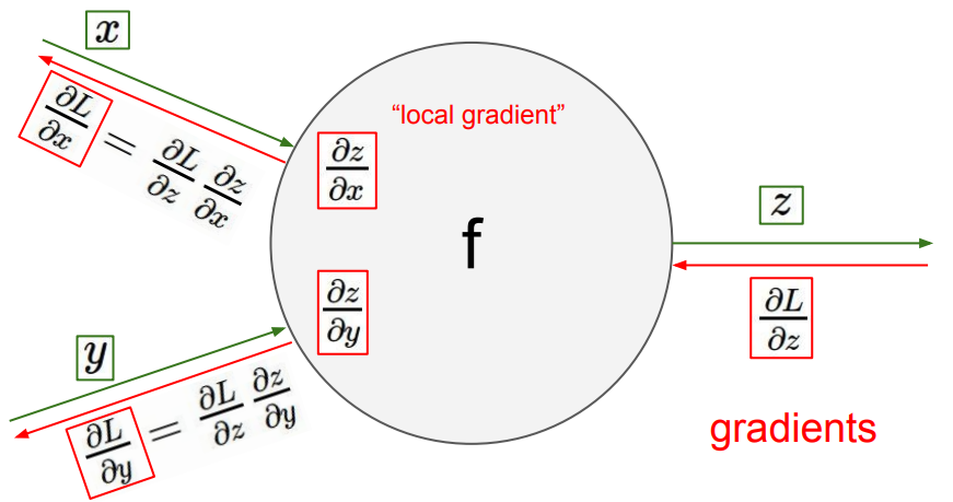
The above picture shows how easy it is to calculate the gradients for the inputs of the neuron given the gradient from the layer ahead. With that in mind, now let us look at a typical convolutional layer.

Convolution of a 3x3 image with a 2x2 filter

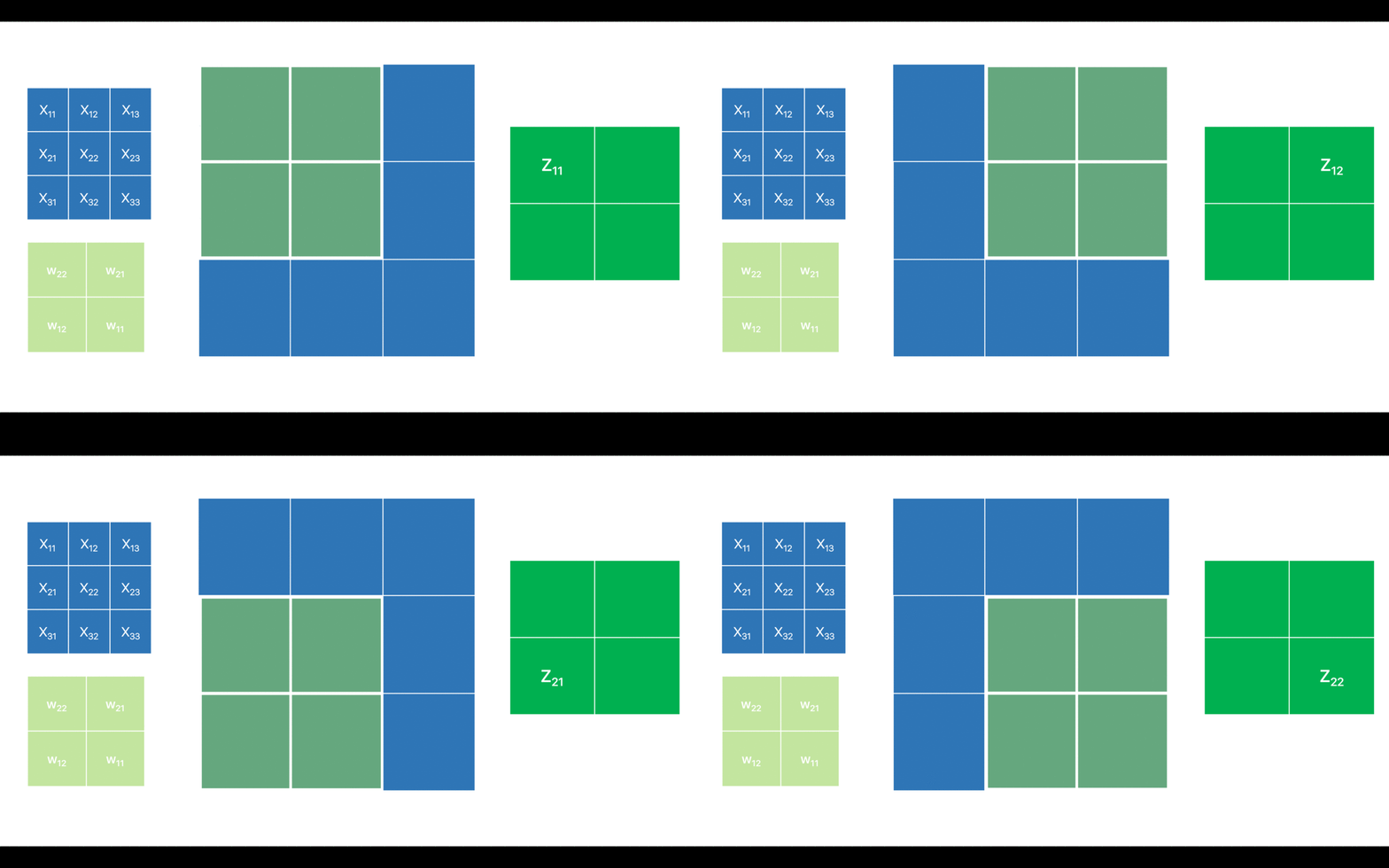
For simplicity, I have only considered one channel. I have denoted the pixel values for the input feature map as ${X}$ which is typically the notation for the input layer. However, that might as well be any intermediate layer ${l}$ for the network and in that case the ${X}$ will be the activations from the previous layer $(l - 1)$ i.e. ${A^{[l - 1]}}$. $Z$ is the output feature map before applying the non-linearity. I have also omitted the ${b}$ (bias term) in order to keep it as comprehensive as possible. 

Now, let’s break down the above convolution operation in an attempt to relate it with the forward pass of a fully connected layer (matrix dot product operation).

Convolution operation - Sparse Connections between weights and feature map

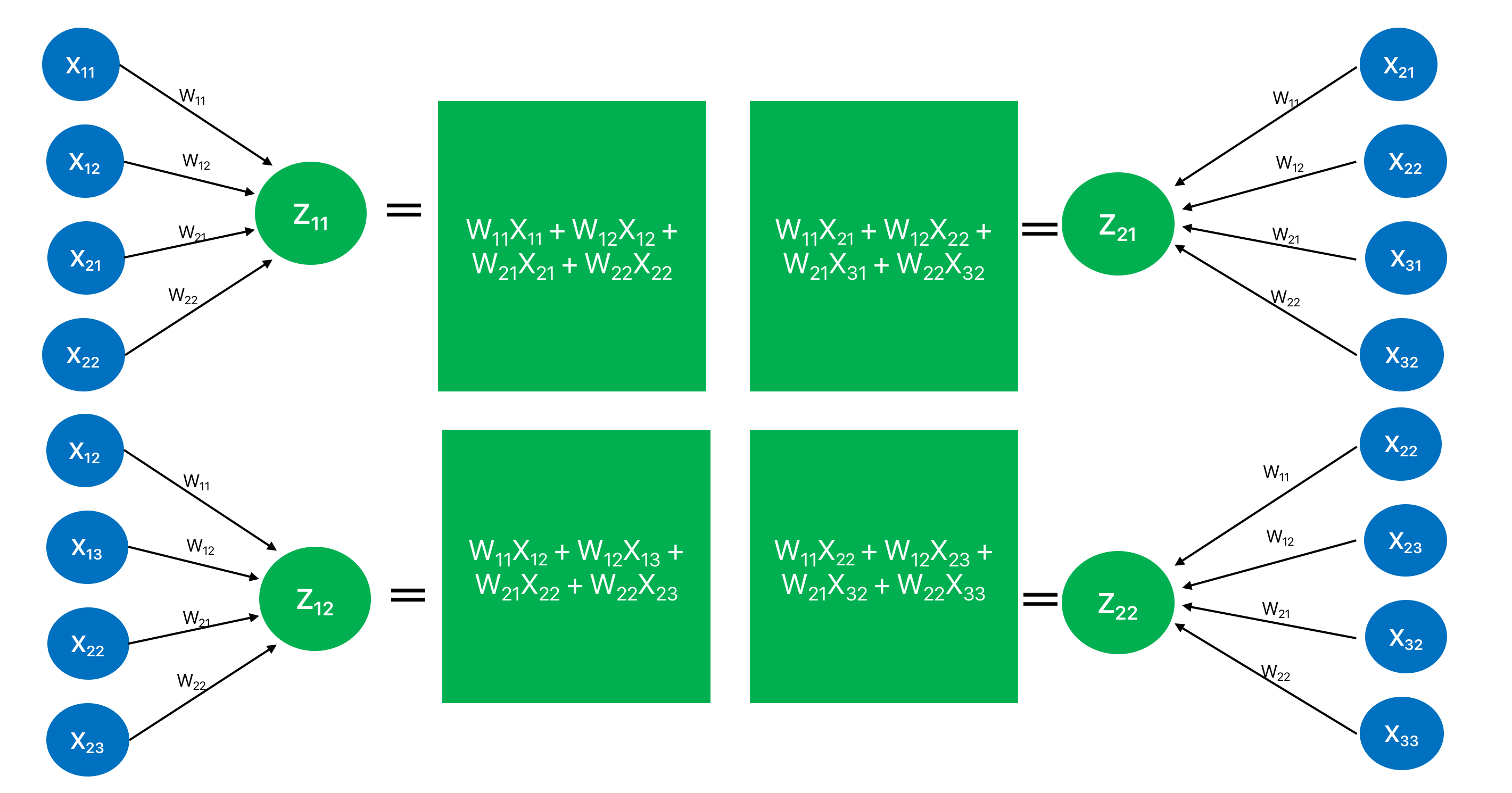
Looks quite similar to a fully-connected neural network, isn’t it? However, by the virtue of sparse connections the output feature map only corresponds to a few (and not all) neurons in the previous layer. Hence, the forward pass in the convnet is pretty straightforward. Before looking into the backward pass though, let’s recap the mantra for the backpropagation which is as follows:

Given $d{Z^{[l]}}$, which is the gradient received at layer ${l}$ from the top of the network, if we can calculate:

1. $d{W^{[l]}}$ (and $d{b^{[l]}}$), which is the weight (and bias) for the ${l^{th}}$ layer and
2. $d{A^{[l - 1]}}$, which is the gradient for the activation map for the previous layer i.e. layer $(l - 1)$ all we are left to do is to iterate back from top to bottom updating the weights through gradient descent. In case you are wondering how the computation of $d{A^{[l - 1]}}$ helps our cause - then let me say this from $d{A^{[l - 1]}}$ you can easily obtain $d{Z^{[l - 1]}}$ with a simple elementwise calculation as below:

and with $d{A^{[l - 1]}}$ we can calculate $d{W^{[l - 1]}}$ and so on.

I just want to cover a couple of more things before looking into the backpropagation for a convolutional layer. This will help you follow more closely. First one is the chain rule of derivative, which I assume, you are already pretty familiar with. However, for the sake of continuity let’s just quickly brush up on that.

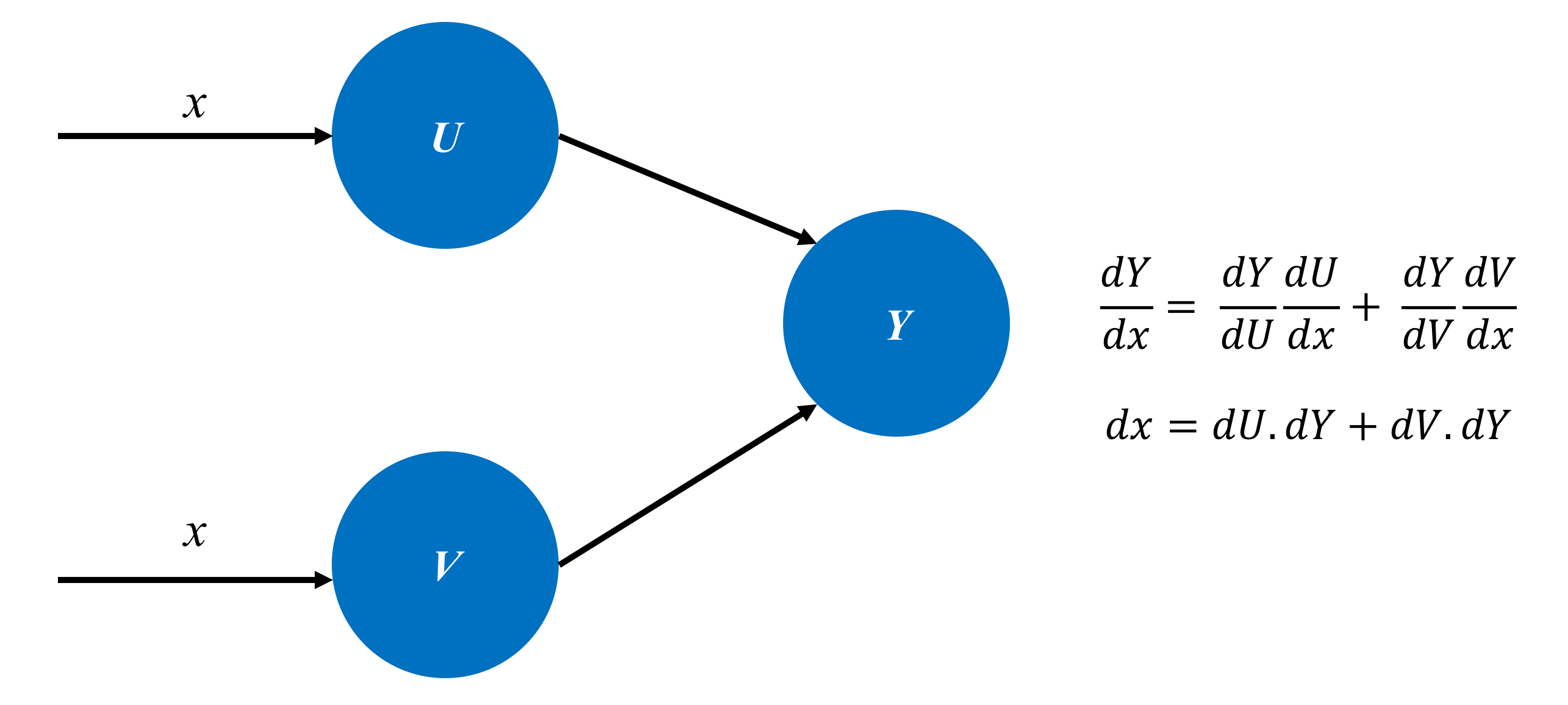
The takeaway from the above picture is that given the gradient of a function (say $dY$), if we want to calculate $dx$ - we have to take into consideration all the connections from ${x}$ to ${Y}$ and take a sum of all the intermediate derivatives.

The last thing that I want to highlight is a full-convolution operation. Most of the time we are talking about convolution we are actually referring to valid convolutions, so let’s take a look how full convolution is different from a valid convolution.

Full Convolution of a 2x2 feature map with a 2x2 filter

Can you guess what would be the size of the output map?

… right, that’s a (3x3) output map which is bigger than the input map. Interesting, isn’t it?

Finally let us put everything together and try to accomplish our goal of computing the backward step for a convolution layer - more specifically calculating $d{W^{[l]}}$ and $d{A^{[l - 1]}}$ given $d{Z^{[l]}}$. To do that let’s first write out the equations for the forward pass:

$${Z_{11}} = {W_{11}}{X_{11}} + {W_{12}}{X_{12}} + {W_{21}}{X_{21}} + {W_{22}}{X_{22}}$$ $${Z_{12}} = {W_{11}}{X_{12}} + {W_{12}}{X_{13}} + {W_{21}}{X_{22}} + {W_{22}}{X_{23}}$$ $${Z_{21}} = {W_{11}}{X_{21}} + {W_{12}}{X_{22}} + {W_{21}}{X_{31}} + {W_{22}}{X_{32}}$$ $${Z_{22}} = {W_{11}}{X_{22}} + {W_{12}}{X_{23}} + {W_{21}}{X_{32}} + {W_{22}}{X_{33}}$$

So given $dZ$ we can calculate $dW$ pretty easily (chain rule to the rescue):

$$d{W_{11}} = d{Z_{11}}{X_{11}} + d{Z_{12}}{X_{12}} + d{Z_{21}}{X_{21}} + d{Z_{22}}{X_{22}}$$ $$d{W_{12}} = d{Z_{11}}{X_{12}} + d{Z_{12}}{X_{13}} + d{Z_{21}}{X_{22}} + d{Z_{22}}{X_{23}}$$ $$d{W_{21}} = d{Z_{11}}{X_{21}} + d{Z_{12}}{X_{22}} + d{Z_{21}}{X_{31}} + d{Z_{22}}{X_{32}}$$ $$d{W_{22}} = d{Z_{11}}{X_{22}} + d{Z_{12}}{X_{23}} + d{Z_{21}}{X_{32}} + d{Z_{22}}{X_{33}}$$

Do you see what’s going on here yet? If not, take a look at the second set of equations more closely. Perhaps one at a time.

Think of the pixels in the input feature map that get affected by the weight term ${W_{11}}$ and you will quickly realise that that’s a (2x2) spatial map in the input feature map as below:

$$\begin{pmatrix}{X_{11}} & {X_{12}}\\\ {X_{21}} & {X_{22}}\end{pmatrix}$$

In the backward pass, we are taking that (2x2) map and convolving that with the $dZ$ which is also (2x2) and the result is our update $d{W_{11}}$. So the locality of connections remain invariant during the backward pass.

So obtaining $dW$ from $dZ$ was quite straightforward. Now let’s find out how we can derive $d{A^{[l - 1]}}$ or $dX$ in our case. We shall think of the connections that we talked about in the chain rule figure. For example, in order to calculate $d{X_{11}}$ - let’s find out first how many connections are their from ${X_{11}}$ to $Z$. Turns out there is only one connection - that is through ${W_{11}}$ to $d{Z_{11}}$. Hence, given $dZ$, we can calculate $d{X_{11}}$ as follows:

$$d{X_{11}} = {W_{11}}d{Z_{11}}$$

What about ${X_{12}}$? There are two connections - ${W_{12}} \to {Z_{11}}$ and ${W_{11}} \to {Z_{12}}$. So, just like above we can obtain:

$$d{X_{12}} = {W_{12}}d{Z_{11}} + {W_{11}}d{Z_{12}}$$

If we calculate the gradients for all the pixels in $X$, we end up with the following matrix:

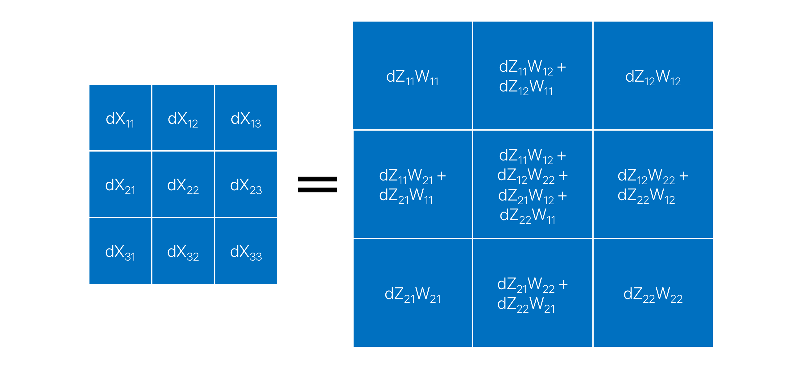
Nothing special so far. Plain simple math. But again take a look at the matrix carefully. Remeber the full convolution still? As it turns out if we rotate the kernel W ${180^o}$ (flip right twice) and perform a full convolution on $dZ$, we get the exact same matrix as $dX$. That is:

$$dX = rot\_180(W) \otimes dZ$$

More generically:

$$d{A^{[l - 1]}} = rot\_180({W^{[l]}}) \otimes d{Z^{[l]}}$$

Which is quite similar to the backpropagation equation for a fully-connected layer - just the weight transpose for the latter is replaced by a convolution in this case.

That’s all for this article. If you have a feedback or question, please feel free to let me know in the comments.